Visualization of gradient descent with one flow line In differential geometry , the Yang–Mills–Higgs flow is a gradient flow described by the Yang–Mills–Higgs equations , hence a method to describe a gradient descent of the Yang–Mills–Higgs action functional. Simply put, the Yang–Mills–Higgs flow is a path always going in the direction of steepest descent, similar to the path of a ball rolling down a hill. This helps to find critical points , called Yang–Mills–Higgs pairs, which solve the Yang–Mills–Higgs equations, as well as to study their stability . Illustratively, they are the points on the hill on which the ball can rest.
The Yang–Mills–Higgs flow is named after Yang Chen-Ning , Robert Mills and Peter Higgs with the former two having formulated the underlying Yang–Mills theory in 1954 and the latter having proposed the coupling to the Higgs field in 1964.
Definition
Let
G
{\displaystyle G}
compact Lie group with Lie algebra
g
{\displaystyle {\mathfrak {g}}}
E
↠
B
{\displaystyle E\twoheadrightarrow B}
principal
G
{\displaystyle G}
with a compact orientable Riemannian manifold
B
{\displaystyle B}
metric
g
{\displaystyle g}
volume form
vol
g
{\displaystyle \operatorname {vol} _{g}}
Ad
(
E
)
:=
E
×
G
g
↠
B
{\displaystyle \operatorname {Ad} (E):=E\times _{G}{\mathfrak {g}}\twoheadrightarrow B}
adjoint bundle .
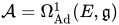
A
=
Ω
Ad
1
(
E
,
g
)
{\displaystyle {\mathcal {A}}=\Omega _{\operatorname {Ad} }^{1}(E,{\mathfrak {g}})}
affine vector space (not canonically) isomorphic to
Ω
1
(
B
,
Ad
(
E
)
)
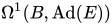
{\displaystyle \Omega ^{1}(B,\operatorname {Ad} (E))}
connections . These are under the adjoint representation
Ad
{\displaystyle \operatorname {Ad} }
g
{\displaystyle {\mathfrak {g}}}
Lie algebra–valued ) differential forms on
E
{\displaystyle E}
B
↪
E
{\displaystyle B\hookrightarrow E}
Ad
(
E
)
{\displaystyle \operatorname {Ad} (E)}
vector bundle –valued) differential forms on
B
{\displaystyle B}
The Yang–Mills–Higgs action functional is given by:[ 1] [ 2]
YMH
:
Ω
Ad
1
(
E
,
g
)
×
Γ
∞
(
B
,
Ad
(
E
)
)
→
R
,
YMH
(
A
,
Φ
)
:=
∫
B
‖
F
A
‖
2
+
‖
d
A
Φ
‖
2
d
vol
g
≥
0.
{\displaystyle \operatorname {YMH} \colon \Omega _{\operatorname {Ad} }^{1}(E,{\mathfrak {g}})\times \Gamma ^{\infty }(B,\operatorname {Ad} (E))\rightarrow \mathbb {R} ,\operatorname {YMH} (A,\Phi ):=\int _{B}\|F_{A}\|^{2}+\|\mathrm {d} _{A}\Phi \|^{2}\mathrm {d} \operatorname {vol} _{g}\geq 0.}
Its first term is also called Yang–Mills action .
Hence the gradient of the Yang–Mills–Higgs action functional gives exactly the Yang–Mills–Higgs equations :
grad
(
YMH
)
(
A
,
Φ
)
1
=
δ
A
F
A
+
[
Φ
,
d
A
Φ
]
,
{\displaystyle \operatorname {grad} (\operatorname {YMH} )(A,\Phi )_{1}=\delta _{A}F_{A}+[\Phi ,\mathrm {d} _{A}\Phi ],}
grad
(
YMH
)
(
A
,
Φ
)
2
=
δ
A
d
A
Φ
.
{\displaystyle \operatorname {grad} (\operatorname {YMH} )(A,\Phi )_{2}=\delta _{A}\mathrm {d} _{A}\Phi .}
For an open interval
I
⊆
R
{\displaystyle I\subseteq \mathbb {R} }
C
1
{\displaystyle C^{1}}
α
:
I
→
A
=
Ω
Ad
1
(
E
,
g
)
{\displaystyle \alpha \colon I\rightarrow {\mathcal {A}}=\Omega _{\operatorname {Ad} }^{1}(E,{\mathfrak {g}})}
φ
:
I
→
Γ
∞
(
B
,
Ad
(
E
)
)
{\displaystyle \varphi \colon I\rightarrow \Gamma ^{\infty }(B,\operatorname {Ad} (E))}
continuously differentiable ) fulfilling:[ 3] [ 4]
α
′
(
t
)
=
−
grad
(
YMH
)
(
α
(
t
)
,
φ
(
t
)
)
1
=
−
δ
α
(
t
)
F
α
(
t
)
−
[
φ
(
t
)
,
d
α
(
t
)
φ
(
t
)
]
{\displaystyle \alpha '(t)=-\operatorname {grad} (\operatorname {YMH} )(\alpha (t),\varphi (t))_{1}=-\delta _{\alpha (t)}F_{\alpha (t)}-[\varphi (t),\mathrm {d} _{\alpha (t)}\varphi (t)]}
φ
′
(
t
)
=
−
grad
(
YMH
)
(
α
(
t
)
,
φ
(
t
)
)
2
=
−
δ
α
(
t
)
d
α
(
t
)
φ
(
t
)
{\displaystyle \varphi '(t)=-\operatorname {grad} (\operatorname {YMH} )(\alpha (t),\varphi (t))_{2}=-\delta _{\alpha (t)}\mathrm {d} _{\alpha (t)}\varphi (t)}
are a Yang–Mills–Higgs flow.
Properties
For a Yang–Mills–Higgs pair
(
A
,
Φ
)
∈
Ω
Ad
1
(
E
,
g
)
×
Γ
∞
(
B
,
Ad
(
E
)
)
{\displaystyle (A,\Phi )\in \Omega _{\operatorname {Ad} }^{1}(E,{\mathfrak {g}})\times \Gamma ^{\infty }(B,\operatorname {Ad} (E))}
For a Yang–Mills–Higgs flow
(
α
,
φ
)
:
I
→
Ω
Ad
1
(
E
,
g
)
×
Γ
∞
(
B
,
Ad
(
E
)
)
{\displaystyle (\alpha ,\varphi )\colon I\rightarrow \Omega _{\operatorname {Ad} }^{1}(E,{\mathfrak {g}})\times \Gamma ^{\infty }(B,\operatorname {Ad} (E))}
(
YMH
∘
(
α
,
φ
)
)
′
(
t
)
=
−
∫
X
‖
α
′
(
t
)
‖
2
+
‖
φ
′
(
t
)
‖
2
d
vol
g
≤
0.
{\displaystyle (\operatorname {YMH} \circ (\alpha ,\varphi ))'(t)=-\int _{X}\|\alpha '(t)\|^{2}+\|\varphi '(t)\|^{2}\mathrm {d} \operatorname {vol} _{g}\leq 0.}
Hence
YMH
∘
(
α
,
φ
)
:
I
→
R
{\displaystyle \operatorname {YMH} \circ (\alpha ,\varphi )\colon I\rightarrow \mathbb {R} }
For any pair
(
A
,
Φ
)
∈
Ω
Ad
1
(
E
,
g
)
×
Γ
∞
(
B
,
Ad
(
E
)
)
{\displaystyle (A,\Phi )\in \Omega _{\operatorname {Ad} }^{1}(E,{\mathfrak {g}})\times \Gamma ^{\infty }(B,\operatorname {Ad} (E))}
(
α
,
φ
)
:
[
0
,
∞
)
→
Ω
Ad
1
(
E
,
g
)
×
Γ
∞
(
B
,
Ad
(
E
)
)
{\displaystyle (\alpha ,\varphi )\colon [0,\infty )\rightarrow \Omega _{\operatorname {Ad} }^{1}(E,{\mathfrak {g}})\times \Gamma ^{\infty }(B,\operatorname {Ad} (E))}
(
α
(
0
)
,
φ
(
0
)
)
=
(
A
,
Φ
)
{\displaystyle (\alpha (0),\varphi (0))=(A,\Phi )}
(
lim
t
→
∞
α
(
t
)
,
lim
t
→
∞
φ
(
t
)
)
{\displaystyle (\lim _{t\rightarrow \infty }\alpha (t),\lim _{t\rightarrow \infty }\varphi (t))}
For a stable Yang–Mills–Higgs pair
(
A
,
Φ
)
∈
Ω
Ad
1
(
E
,
g
)
×
Γ
∞
(
B
,
Ad
(
E
)
)
{\displaystyle (A,\Phi )\in \Omega _{\operatorname {Ad} }^{1}(E,{\mathfrak {g}})\times \Gamma ^{\infty }(B,\operatorname {Ad} (E))}
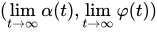
neighborhood so that every unique Yang–Mills–Higgs flow
(
α
,
φ
)
:
[
0
,
∞
)
→
Ω
Ad
1
(
E
,
g
)
×
Γ
∞
(
B
,
Ad
(
E
)
)
{\displaystyle (\alpha ,\varphi )\colon [0,\infty )\rightarrow \Omega _{\operatorname {Ad} }^{1}(E,{\mathfrak {g}})\times \Gamma ^{\infty }(B,\operatorname {Ad} (E))}
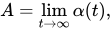
A
=
lim
t
→
∞
α
(
t
)
,
{\displaystyle A=\lim _{t\rightarrow \infty }\alpha (t),}
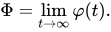
Φ
=
lim
t
→
∞
φ
(
t
)
.
{\displaystyle \Phi =\lim _{t\rightarrow \infty }\varphi (t).}
A generalization of the Yang–Mills–Higgs flow is the Ginzburg–Landau flow, named after Vitaly Ginzburg and Lev Landau , with an additional potential term for the Higgs field.
Literature
Zhang, Pan (2020-03-30). "Gradient Flows of Higher Order Yang-Mills-Higgs Functionals". arXiv :2004.00420 math.DG ]. Changpeng Pan, Zhenghan Shen, Pan Zhang (2024). "The Limit of the Yang-Mills-Higgs Flow for twisted Higgs pairs". International Journal of Geometric Methods in Modern Physics . 21 (4) 2450075: 2450075– 33. arXiv :2301.02552 Bibcode :2024IJGMM..2150075P . doi :10.1142/S0219887824500750 . {{cite journal}}: CS1 maint: multiple names: authors list (link)
See also
External links
References
^ Zhang 2020, Eq. (1.1)
^ Changpeng, Zhenghan & Zhang 2023, Eq. (1.2)
^ Zhang 2020, Eq. (1.3)
^ Changpeng, Zhenghan & Zhang 2023, Eq. (1.4)






![{\displaystyle \operatorname {grad} (\operatorname {YMH} )(A,\Phi )_{1}=\delta _{A}F_{A}+[\Phi ,\mathrm {d} _{A}\Phi ],}](./_assets_/eb734a37dd21ce173a46342d1cc64c92/d695e297192ca185d906a89a1fb1664367bc1b8d.svg)





![{\displaystyle \alpha '(t)=-\operatorname {grad} (\operatorname {YMH} )(\alpha (t),\varphi (t))_{1}=-\delta _{\alpha (t)}F_{\alpha (t)}-[\varphi (t),\mathrm {d} _{\alpha (t)}\varphi (t)]}](./_assets_/eb734a37dd21ce173a46342d1cc64c92/bc3dcececd6ef219a30a2e10e5d326723dedeec9.svg)